Table of Contents
Using R for data analysis.
This page shows how to connect R scripts to XGAP. See RqtlIntegration for integration with the RqtlPackage.
Connecting R to XGAP
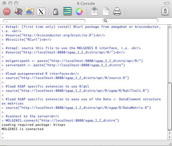
This example shows how to connect to XGAP from within R:
- In the XGAP user interface, go to "Programming interfaces".
- Click the link at "Access from the R project: source the file at api/R".
- Select and copy all the commands
- Open R, and paste the commands. If you haven't installed RCurl, please do so now. (See "step 1" in the sourced code)
Retrieving annotation data
This examples show how to retrieve annotation data from XGAP (except data matrices). We will use the example of 'marker'.
- Retrieve annotations use find.*. For example:
allMarkers <- find.marker()
Tip: if you only type 'find.' and then push 'TAB' you will see all find.* functions available.
- One can use the R function dim() to see the dimensions of this object. In this example, there are 251 markers with 17 attributes each.
dim(allMarkers)
Result:
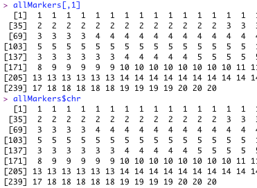
- By selecting the first column, you get to see the chromosome attribute for each marker:
Use:
allMarkers[,1]
It is even easier to retrieve a particular column using the '$ plus column name' notation: Use:
allMarkers$chrResult:
- You can select the first marker by picking the first row:
Use:
allMarkers[1,]
- And only name of this marker by combining the syntaxes:
Use:
allMarkers[1,]$name
- The '$' notation does not work for multiple columns. So, if you wish to see specific attributes for all markers, you have to pass the column names as follows:
Use:
allMarkers[,c("id","chr","name")]Result:
Retrieving data matrices
Data is stored in XGAP in the form of matrices. The following examples show how to retrieve these data sets into R.
- First, get a list of all data matrices available in the database. Adding some more arguments will limit the output shown to only data.id, name and investigation name.
Use:
find.data()[,c("id","name","investigation_name")]Result:
- Select and retrieve the data for one data matrix. In this example let's pick the metabolite expression matrix which had id 6. Then you can download it like this:
data <- find.datamatrix(6)
- Like with annotation data above, one can also inspect the size of the downloaded matrix:
dim(data)
Result:
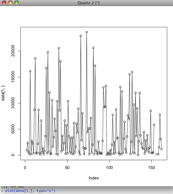
- Now make an 'overplotted' plot of the first column. (In this case: the first 1 trait, for all individuals)
plot(data[1,], type="o")
Result:
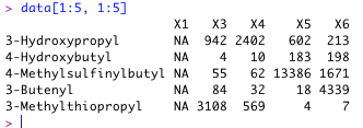
- In contrast with annotations, data matrices also have row headers, next to column headers. You can check this by using functions like colnames(), rownames(). Note that you can use these to select a subset of the matrix:
data[1:5, 1:5]
Result:
Uploading annotations
Get a list of the investigations with attributes 'id' and 'name'. In this case, we use the 'MetaNetwork' investigation which has id = 1.
Use:
find.investigation()[,c("id", "name")]
Suppose we would like to add a pseudomarker during a QTL investigation. We can easily add a single marker by using add.marker:
Use:
add.marker(name="loc50.0", cm="50.0", chr="2", investigation_id=1)
It's also possible to add a list of markers at once. This can be done by constructing a dataframe. Use 'colnames' to set the attributes. An example:
Use:
pseudo <- NULL
pseudo <- rbind(pseudo, c("loc0.0","0.0","14", 1))
pseudo <- rbind(pseudo, c("loc10.0","10.0","15", 1))
pseudo <- rbind(pseudo, c("loc22.0","22.0","16", 1))
colnames(pseudo) <- c("name", "cm", "chr", "investigation")
add.marker(pseudo)
You can add the result to a variable so you can use its properties (eg. the assigned id in the database) later on.
Use:
myPseudo = add.marker(pseudo);
myPseudo #print the list of markers
Uploading data matrices
Option A
This is the easier way, using a custom function.
Creata a matrix and add two rows with, for example, genotyping data:
Use:
data <- NULL
data <- rbind(data, c("A", "B"))
data <- rbind(data, c("B", "A"))
If the individuals and markers are not present in the database, add them first.
Use:
marker1 = add.marker(name="myMarker1", cm="10.0", chr="2", investigation_id=1)
marker2 = add.marker(name="myMarker2", cm="20.0", chr="2", investigation_id=1)
ind1 = add.individual(name="myInd1", investigation_id=1)
ind2 = add.individual(name="myInd2", investigation_id=1)
Now add reference to the individuals of which the genotypes are measured, and ofcourse the markers that have been genotyped. Be careful to not switch 'rows' with 'columns'.
Use:
colnames(data) <- c("myInd1", "myInd2")
rownames(data) <- c("myMarker1", "myMarker2")
Now we add this matrix by using the custom 'add.datamatrix' function. Several attributes need to be entered, for example the name and row/column type of the matrix. We know the investigation to add this matrix to has id = 1.
Use:
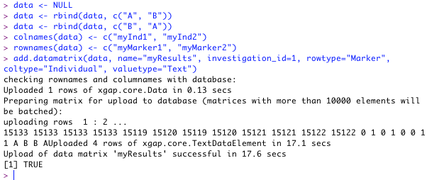
add.datamatrix(data, name="myResults", investigation_id=1, rowtype="Marker", coltype="Individual", valuetype="Text")
When successful, something like this will appear:
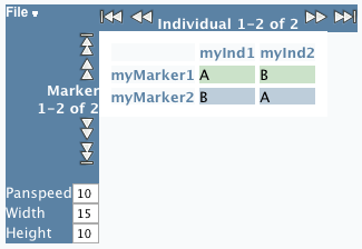
You can inspect the result in the user interface:
Option B
This is the harder way, performing several manual steps by yourself.
First, add a Data object. This is basically the description of a datamatrix. We add it under the investigation with id = 1. Say we add genotyping data. In this case, the rowtype will be 'marker', the columns 'individual. We add two rows and two columns. The values will be text. (eg. 'A' or 'B')
Use:
data <- add.data(name = "myResults", investigation_id=1, rowtype="Marker",coltype="Individual",totalrows=2,totalcols=2,valuetype="Text")
Now lets add elements which we will refer to. This can also be existing elements ofcourse. We add two markers with some information, and two individuals with just names.
Use:
marker1 = add.marker(name="myMarker1", cm="10.0", chr="2", investigation_id=1)
marker2 = add.marker(name="myMarker2", cm="20.0", chr="2", investigation_id=1)
ind1 = add.individual(name="myInd1", investigation_id=1)
ind2 = add.individual(name="myInd2", investigation_id=1)
We can now add the actual values. Here we use 'add.textdataelement' contrary to 'add.decimaldataelement' because the valuetype for the matrix is text. From the existing 'data' object, we get the id to add the element to. We do the same for the markers and individuals. Then we indicate the position of the elements in the matrix using indices and finally the value of the element.
Use:
add.textdataelement(data_id=data$id, row_id=marker1$id, col_id=ind1$id, rowindex=0, colindex=0, value="A")
add.textdataelement(data_id=data$id, row_id=marker1$id, col_id=ind2$id, rowindex=0, colindex=1, value="B")
add.textdataelement(data_id=data$id, row_id=marker2$id, col_id=ind1$id, rowindex=1, colindex=0, value="B")
add.textdataelement(data_id=data$id, row_id=marker2$id, col_id=ind2$id, rowindex=1, colindex=1, value="A")
Attachments (10)
- R1.png (71.4 KB) - added by 16 years ago.
- R2.png (10.8 KB) - added by 16 years ago.
- R3.png (16.1 KB) - added by 16 years ago.
- R4.png (30.8 KB) - added by 16 years ago.
- R5.png (22.1 KB) - added by 16 years ago.
- R6.png (3.7 KB) - added by 16 years ago.
- R7.png (82.6 KB) - added by 16 years ago.
- R8.png (10.4 KB) - added by 16 years ago.
- R9.png (18.3 KB) - added by 16 years ago.
- R10.png (26.9 KB) - added by 16 years ago.
Download all attachments as: .zip
